
Phthalate Exposure in U.S. Women of Reproductive Age - an NHANES Review, Part I
Motivation
Perhaps I’m the type of person that worries excessively about things outside of their control, but I’ve long been concerned about plastics leaching into our bodies from things like food packaging and personal care products.
Some of these anxieties might be justified. A recent analysis of bio-specimen data from the National Health and Nutrition Examination Survey NHANES, the largest annual survey of the United States population, found nearly ubiquitous exposure to phthalates (Zota et al, 2014). This is particularly concerning for pregnant women because studies have found adverse effects, including shorter pregnancy duration and decreased head circumference (Polanska et al, 2016), as well as endocrine disrupting effects in males, including decreased anogenital distance (animal study) (Swan et al, 2005) and damage to sperm DNA (Duty et al, 2003). So how concerned should we be?
After reviewing the literature, I wanted to answer the following questions:
- What phthalates are present in women in the US, what are the average levels of these phthalates, and how have these levels changed over time?
- Are phthalate levels disproportionately distributed through the population? Namely, is there an association with phthalates and socioeconomic status?
We’ll cover question 1 here and question 2 in the next post.
Background
Before we dive in to the data, we need a bit of priming on what phthalates are and why they’re important. Phthalates are the most common category of industrial plasticizers (chemicals that alter the flexibility and rigidity of plastics) in use today. Due to their widespread presence in manufacturing, the metabolites of these chemicals (i.e the breakdown products when they enter the body) are now ubiquitously detectable in humans in the United States (Zota et al, 2014). Phthalates are of particular concern in women of reproductive age because they can easily cross the placenta and interact with fetal development during critical windows of pregnancy (Polanska et al, 2016). Previous studies have established detrimental defects on reproductive system development in fetuses exposed to phthalates (Swan et al, 2005).
Applications of phthalates range from building materials, including flooring and adhesives, to personal care products, including nail polish and shampoo CDC. High molecular weight phthalates like butylbenzyl phthalate (BBzP), di(2-ethylhexyl) phthalate (DEHP) and diisononyl phthalate (DiNP) are commonly found in building materials. Low molecular weight materials like diethyl phthalate (DEP), di-n-butyl phthalate (DnBP) are more commonly found in personal care products and medications (Zota et al, 2014).
Although several studies have been conducted using cohorts, a powerful tool at our disposal is NHANES. This national survey has been performed annually by the CDC since 1960, provides a large sample size (about 10,000 participants per year), and assesses a very wide range of health factors including demographics, diet, chronic health conditions, and biomarkers in blood and urine. Because of its breadth and large sample size, NHANES provides rich datasets for studying associations between these health attributes.
Analysis
Although there is a library for analyzing NHANES in R (aptly named RNHANES), if you work with it long enough, you will notice that only some cycles and variables are available. I spent more time than I care to admit wrangling with this library, and ultimately concluded it would not give me what I needed. Instead, I downloaded the SAS export files from CDC’s NHANES website and imported them to R using the foreign library. Below are the setup, import, and tidying steps I used.
Data Preparation
Libraries
library(tidyverse)
library(foreign)
library(stats)
library(viridis)
library(survey)
library(plotly)
library(kableExtra)
library(gridExtra)
library(sjPlot)
Data Import
First, we read in NHANES cycles 2003 - 2004, 2005 - 2006, 2007 - 2008, 2009 - 2010, 2011 - 2012, 2013 - 2014, and 2015-2016. As of June 2020, phthalate data for 2017 - 2018 was not yet available. The NHANES datasets used are Demographics (DEMO) and Phthalates and Plasticizers Metabolites - Urine (PHTHTE). For the 2015-2016 cycle we also need the Albumin & Creatinine (ALB_CR_I) file since creatinine data were removed from the phthalates files during this cycle (more on creatinine below).
# reading in 2003 - 2004 data
demo_03_04 = read.xport("./data/phthalates/2003_2004_DEMO_C.XPT")
phthalate_03_04 = read.xport("./data/phthalates/2003_2004_PHTHTE_C.XPT.txt")

# reading in 2005 - 2006 data
demo_05_06 = read.xport("./data/phthalates/2005_2006_DEMO_D.XPT")
phthalate_05_06 = read.xport("./data/phthalates/2005_2006_PHTHTE_D.XPT.txt")

# reading in 2007 - 2008 data
demo_07_08 = read.xport("./data/phthalates/2007_2008_DEMO_E.XPT")
phthalate_07_08 = read.xport("./data/phthalates/2007_2008_PHTHTE_E.XPT.txt")

# reading in 2009 - 2010 data
demo_09_10 = read.xport("./data/phthalates/2009_2010_DEMO_F.XPT")
phthalate_09_10 = read.xport("./data/phthalates/2009_2010_PHTHTE_F.XPT.txt")

# reading in 2011 - 2012 data
demo_11_12 = read.xport("./data/phthalates/2011_2012_DEMO_G.XPT.txt")
phthalate_11_12 = read.xport("./data/phthalates/2011_2012_PHTHTE_G.XPT.txt")

# reading in 2013 - 2014 data
demo_13_14 = read.xport("./data/phthalates/2013_2014_DEMO_H.XPT.txt")
phthalate_13_14 = read.xport("./data/phthalates/2013_2014_PHTHTE_H.XPT.txt")

# reading in 2015 - 2016 data (note change in creatinine source file for this cycle)
demo_15_16 = read.xport("./data/phthalates/2015_2016_DEMO_I.XPT.txt")
phthalate_15_16 = read.xport("./data/phthalates/2015_2016_PHTHTE_I.XPT.txt")
creat_15_16 = read.xport("./data/phthalates/2015_2016_ALB_CR_I.XPT.txt")
Data Tidy
Next we’ll bind the data files for each cycle using left-joins, merging on the unique identifier SEQN.
data_03_04 =
  left_join(demo_03_04, phthalate_03_04, by = "SEQN") %>%
  mutate(cycle = "2003-2004")

data_05_06 =
  left_join(demo_05_06, phthalate_05_06, by = "SEQN") %>%
  mutate(cycle = "2005-2006")

data_07_08 =
  left_join(demo_07_08, phthalate_07_08, by = "SEQN") %>%
  mutate(cycle = "2007-2008")

data_09_10 =
  left_join(demo_09_10, phthalate_09_10, by = "SEQN") %>%
  mutate(cycle = "2009-2010")

data_11_12 =
  left_join(demo_11_12, phthalate_11_12, by = "SEQN") %>%
  mutate(cycle = "2011-2012")

data_13_14 =
  left_join(demo_13_14, phthalate_13_14, by = "SEQN") %>%
  mutate(cycle = "2013-2014")

data_15_16 =
  left_join(demo_15_16, phthalate_15_16, by = "SEQN") %>%
  left_join(creat_15_16, by = "SEQN") %>%
  mutate(cycle = "2015-2016")

all_data =
  bind_rows(data_03_04, data_05_06, data_07_08, data_09_10, data_11_12, data_13_14, data_15_16)
Variables Used
Next, we’ll select the variables we want. We will choose 12 phthalates measured in NHANES between 2003 and 2016, as well as urinary creatinine URXUCR. The latter is a constant byproduct of metabolic activities and is often used to measure urinary dilution.
NHANES takes biosample data for about 1/3 of the survey participants, so we will remove observations with missing phthalate data. We will restrict analysis to female respondents between the ages of 20 and 44, which we’ll take to mean reproductive age in this analysis. We will also include age and socioeconomic measures to be used in Question 2.
Below are the NHANES variables used, along with abbreviations for phthalate names. More intuitive variable names are assigned the subsequent code chunk.
SEQN: Unique NHANES identifierRIAGENDR: GenderRIDAGEYR: AgeRIDRETH1: EthnicityDMDEDUC2: EducationDMDMARTL: Marital StatusINDHHIN2: Annual household income (cycles 2007-2008, 2009-2010, 2011-2012, 2013-2014, 2015-2016)INDFMIN2: Annual family income (cycles 2007-2008, 2009-2010, 2011-2012, 2013-2014, 2015-2016)INDHHINC: Annual household income (cycles 2003-2004, 2005-2006)INDFMINC: Annual family income (cycles 2003-2004, 2005-2006)WTMEC2YR,SDMVPSU,SDMVSTRA: Survey weighting variables, addressed in Question 2 belowURXUCR: Urinary creatinineURXCNP: Mono(carboxyisononyl) phthalate (MCNP) (ng/mL)URXCOP: Mono(carboxyisoctyl) phthalate (MCOP) (ng/mL)URXMNP: Mono-isononyl phthalate (MiNP) (ng/mL)URXECP: Mono-2-ethyl-5-carboxypentyl phthalate (MECPP) (ng/mL)URXMHH: Mono-(2-ethyl-5-hydroxyhexyl) phthalate (MEHHP) (ng/mL)URXMHP: Mono-(2-ethyl)-hexyl phthalate (MEHP) (ng/mL)URXMOH: Mono-(2-ethyl-5-oxohexyl) phthalate (MEOHP) (ng/mL)URXMBP: Mono-n-butyl phthalate (MnBP) (ng/mL)URXMEP: Mono-ethyl phthalate (MEP) (ng/mL)URXMIB: Mono-isobutyl phthalate (MiBP) (ng/mL)URXMC1: Mono-(3-carboxypropyl) phthalate (MCPP) (ng/mL)URXMZP: Mono-benzyl phthalate (MBzP) (ng/mL)
# select variables of interest, drop every observation without biomarker data, filter out women aged 20-44, and consolidate household and family income variables
all_data =
  all_data %>%
  select(SEQN, cycle, RIAGENDR, RIDAGEYR, RIDRETH1, DMDEDUC2, DMDMARTL, INDHHINC, INDFMINC, INDHHIN2, INDFMIN2, WTMEC2YR, SDMVPSU, SDMVSTRA, URXUCR, URXECP, URXMBP, URXMC1, URXMEP, URXMHH, URXMHP, URXMIB, URXMOH, URXMZP, URXMNP, URXCOP, URXMNP, URXCNP) %>%
  drop_na(URXMEP) %>%
  rename(gender = RIAGENDR, age = RIDAGEYR, ethnicity = RIDRETH1, education = DMDEDUC2, marital_status = DMDMARTL, creatinine = URXUCR, mecpp = URXECP, mnbp = URXMBP, mcpp = URXMC1, mep = URXMEP, mehhp = URXMHH, mehp = URXMHP, mibp = URXMIB, meohp = URXMOH, mbzp = URXMZP, mcnp = URXCNP, mcop = URXCOP, minp = URXMNP) %>%
  filter(gender == 2, age %in% (20:44)) %>%
  mutate(
    household_income = if_else(cycle %in% c("2003-2004", "2005-2006"), INDHHINC, INDHHIN2),
    family_income = if_else(cycle %in% c("2003-2004", "2005-2006"), INDFMINC, INDFMIN2)
    ) %>%
  select(-c(INDHHINC, INDHHIN2, INDFMINC, INDFMIN2))
Finally, we will add variables for creatinine-adjusted phthalate concentrations. There is, however, a units mismatch we’ll need to deal with. Creatinine is measured in mg/dL and all phthalate biomarkers are measured in ng/mL. Creatinine adjusted measures are reported here (and often in literature) in units of \(\)g phthalate/g creatinine. To get to these final units, we multiply the phthalate concentration by 100 and divide by creatinine 1. Adjusted values are denoted with a _c.
all_data_c =
  all_data %>%
  mutate(mecpp_c = 100*mecpp/creatinine,
         mnbp_c = 100*mnbp/creatinine,
         mcpp_c = 100*mcpp/creatinine,
         mep_c = 100*mep/creatinine,
         mehhp_c = 100*mehhp/creatinine,
         mehp_c = 100*mehp/creatinine,
         mibp_c = 100*mibp/creatinine,
         meohp_c = 100*meohp/creatinine,
         mbzp_c = 100*mbzp/creatinine,
         mcnp_c = 100*mcnp/creatinine,
         mcop_c = 100*mcop/creatinine,
         minp_c = 100*minp/creatinine)
Question 1: What phthalates are present in women in the US, what are the average levels of these chemicals, and how have these levels changed over time?
After I set about answering the first question, I realized that the most interesting part is the temporal aspect. If there were spikes in certain phthalates, for instance, that would narrow my focus going forward. Conversely, if phthalates were steadily decreasing in the population, maybe this would assuage my anxieties and I could find something else to worry about. Either way, I decided to tackle this question first. I used a spaghetti plot to visualize phthalates over the seven cycles of data and added ggplotly interactivity to help distinguish one line from the other.
means_c =
  all_data_c %>%
  select(-c(gender:mbzp), -c(SEQN, mcnp, mcop, mcnp_c, mcop_c)) %>%
  pivot_longer(c(mecpp_c:minp_c), names_to = "chemical_c", values_to = "value") %>%
  drop_na() %>%
  mutate(chemical_c = recode(chemical_c,
                           "mecpp_c"= "Mono-2-ethyl-5-carboxypentyl phthalate (MECPP_c)",
                           "mnbp_c"= "Mono-n-butyl phthalate (MnBP_c)",
                           "mcpp_c"= "Mono-(3-carboxypropyl) phthalate (MCPP_c)",
                           "mep_c"= "Mono-ethyl phthalate (MEP_c)",
                           "mehhp_c"= "Mono-(2-ethyl-5-hydroxyhexyl) phthalate (MEHHP_c)",
                           "mehp_c"= "Mono-(2-ethyl)-hexyl phthalate (MEHP_c)",
                           "mibp_c"= "Mono-isobutyl phthalate (MiBP_c)",
                           "meohp_c"= "Mono-(2-ethyl-5-oxohexyl) phthalate (MEOHP_c)",
                           "mbzp_c"= "Mono-benzyl phthalate (MBzP_c)",
                           "mcnp_c"= "Mono(carboxyisononyl) phthalate (MCNP_c)",
                           "mcop_c"= "Mono(carboxyisoctyl) phthalate (MCOP_c)",
                           "minp_c"= "Mono-isononyl phthalate (MiNP_c)")) %>%
  group_by(cycle, chemical_c) %>%
  summarize(mean_c = mean(value), n = n(), sd = sd(value), median_c = median(value), iqr_c = IQR(value))

sp_plot =
  means_c %>%
  ggplot(aes(x = cycle, y = mean_c)) +
  geom_line(aes(group = chemical_c, color = chemical_c))+
  labs(
    title = "Figure 1: Mean creatinine-adjusted phthalate concentration \n by NHANES cycle in women aged 20 - 44 (n = 2,754)",
    x = "NHANES Cycle",
    y = "Phthalate oncentration (ug/g creatinine)"
  ) +
  theme(text = element_text(size = 9)) + scale_colour_viridis_d(option = "inferno")

ggplotly(sp_plot)
Immediately, it’s clear that MEP stands out. Peaking during the 2005-2006 cycle at 628.92 \(\)g creatinine, MEP represented more than six times the biomarker concentration of the next highest phthalate, MECPP. Following the peak, the concentration fell sharply in 2007-2008 and continued to decline through next four cycles. All other phthalates also show a general decline over time.
What’s special about MEP and why did it decline so sharply? At first, I thought maybe there was an issue with the data. Perhaps an error in the 2005-2006 cycle, or, since we looked at means, some extremely influential outliers that drove the mean upward. However, calculating the median (a statistic not susceptible to outliers) below confirms that MEP is still the highest phthalate by far, measuring more than 4 times the mean of the next highest phthalate, MECPP.
means_c %>%
  filter(cycle == "2005-2006") %>%
  select(cycle, chemical_c, median_c)
## # A tibble: 10 × 3
## # Groups: cycle [1]
## cycle chemical_c median_c
## <chr> <chr> <dbl>
## 1 2005-2006 Mono-(2-ethyl-5-hydroxyhexyl) phthalate (MEHHP_c) 18.7
## 2 2005-2006 Mono-(2-ethyl-5-oxohexyl) phthalate (MEOHP_c) 13.2
## 3 2005-2006 Mono-(2-ethyl)-hexyl phthalate (MEHP_c) 3.13
## 4 2005-2006 Mono-(3-carboxypropyl) phthalate (MCPP_c) 1.84
## 5 2005-2006 Mono-2-ethyl-5-carboxypentyl phthalate (MECPP_c) 29.8
## 6 2005-2006 Mono-benzyl phthalate (MBzP_c) 8.76
## 7 2005-2006 Mono-ethyl phthalate (MEP_c) 132.
## 8 2005-2006 Mono-isobutyl phthalate (MiBP_c) 5.87
## 9 2005-2006 Mono-isononyl phthalate (MiNP_c) 0.917
## 10 2005-2006 Mono-n-butyl phthalate (MnBP_c) 20.4Now that we’ve gone through this sanity check, we’re back to figuring out why MEP stands out from the pack. And to be honest, after scouring the bowels of the internet, I didn’t find a smoking gun. We do know that MEP is the primary metabolite of Diethyl Phthalate (DEP), which, like other phthalates, is used as a plasticizer for rigid materials including toys and toothbrushes. Unlike other phthalates, however, DEP is also used as a solvent in liquid cosmetics and perfumes. As such, the route of exposure is not only oral but also topical, perhaps explaining some of this unique trajectory.
At this point, we might want to pull some information on industrial DEP usage in the US over the past 15 years and perhaps do some research on whether industry/policy changes circa 2005. Ah, but not so fast… After going down this rabbit hole, I learned some enlightening/frustrating information about the history of chemical reporting policies in the US. If this isn’t your cup of tea, feel free to skip to the following section.
A brief historical interlude
In 1976, Congress passed the Toxic Substances Control Act, which sought to measure and regulate industrial usage of chemicals deemed to pose “unreasonable risk” to humans and the environment.
The EPA was tasked with administration of the act and since passage, an inventory of about 84,000 chemicals has been established. In short, the inventory is problematic. First, it’s only updated every four years. Second, it gives exemptions to smaller manufacturers and an ever-growing list of exempt chemicals. Finally (and most importantly), quantities are often reported in extremely wide ranges (“1,000,000 - <20,000,000 lbs” was an entry I saw in the 2016 data…) (Zota et al, 2014, Sciences et al).
Basically, I once assumed that some governing body has a solid grasp on the quantities and types of chemicals used in the US. I no longer assume this.
In another facet of this regulatory picture, we have the Consumer Product Safety Improvement Act of 2008. The act focuses on toxic substances in childrens’ toys and banned presence of certain phthalates (check out this disturbing pile of dolls seized by US Customs in 2013 due to excess phthalate levels).
One might think this would provide some clues on why MEP declined, but the timing doesn’t work out- the act went into effect in 2009 and our trend started in 2004/2005. Additionally, DEP is not included in the scope, it’s hard to ascribe the act as the root cause. It is possible, however, that the industry responded to pressure from advocacy groups and consumers, or in anticipation of further bans, and undertook formulation changes outside of (and prior to) passage of the act.
Back to the numbers
Up until now, we’ve explored the temporal trends of common phthalates and did a bit of unsuccessful (but fun?) digging through the exciting world of toxic chemical legislative history. Now we will backtrack and summarize the average levels, as posed by Question 1.
We proceed to summarizing the raw and creatinine-adjusted values from the 2015-2016 NHANES cycle. Mean and median values for both measures are reported in Table 1 below. Both are shown because there is a high degree of right-skew in the data. To illustrate this, here is a quick histogram of unadjusted MEP levels.
all_data %>%
  ggplot(aes(x = mep)) +
  geom_histogram(binwidth = 500) +
  labs(x = "Unadjusted MEP (ng/mL)",
       title = "Figure 2: MEP Histogram")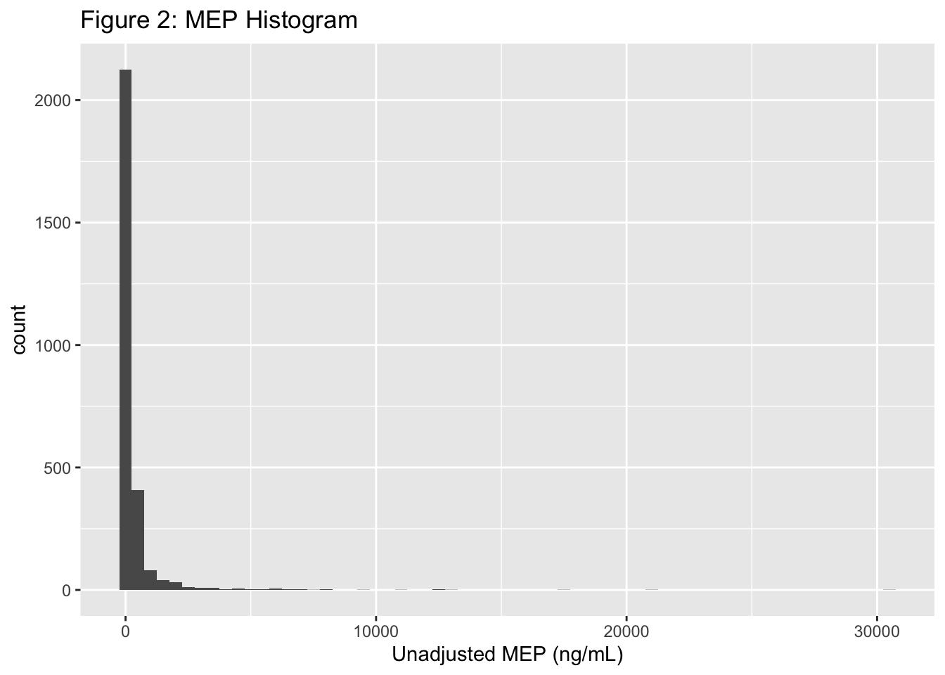
This right-skew is predictable - most people (thankfully) have very low levels of urinary MEP. As such, the median is a better measure of central tendency than the mean. We will look at both since some of the literature I reference below uses mean values and keeping the means will allow for comparison.
# calculating means and medians for phthalate values, not adjusted for creatinine
means_raw =
all_data_c %>%
  filter(cycle == "2015-2016") %>%
  select(-c(gender:creatinine), -SEQN, -c(mecpp_c:minp_c)) %>%
  pivot_longer(c(mecpp:mcnp), names_to = "chemical", values_to = "value") %>%
  drop_na() %>%
  mutate(chemical = recode(chemical,
                           "mecpp"= "Mono-2-ethyl-5-carboxypentyl phthalate (MECPP)",
                           "mnbp"= "Mono-n-butyl phthalate (MnBP)",
                           "mcpp"= "Mono-(3-carboxypropyl) phthalate (MCPP)",
                           "mep"= "Mono-ethyl phthalate (MEP)",
                           "mehhp"= "Mono-(2-ethyl-5-hydroxyhexyl) phthalate (MEHHP)",
                           "mehp"= "Mono-(2-ethyl)-hexyl phthalate (MEHP)",
                           "mibp"= "Mono-isobutyl phthalate (MiBP)",
                           "meohp"= "Mono-(2-ethyl-5-oxohexyl) phthalate (MEOHP)",
                           "mbzp"= "Mono-benzyl phthalate (MBzP)",
                           "mcnp"= "Mono(carboxyisononyl) phthalate (MCNP)",
                           "mcop"= "Mono(carboxyisoctyl) phthalate (MCOP)",
                           "minp"= "Mono-isononyl phthalate (MiNP)")) %>%
  group_by(chemical) %>%
  summarize(mean = mean(value), median = median(value)) %>%
  mutate(id = row_number())

# Calculating means and medians for adjusted values
means_c_15_16 =
  means_c %>%
  filter(cycle == "2015-2016") %>%
  mutate(id = row_number()) %>%
  select(id, chemical_c, mean_c, median_c)

# joining adjusted and un-adjusted into one table
left_join(means_c_15_16, means_raw, by = "id") %>%
  select(c("cycle", "chemical", "mean", "median", "mean_c", "median_c")) %>%
  rename("Chemical" = "chemical", "Adjusted Mean" = "mean_c", "Adjusted Median" = "median_c", "Mean" = "mean", "Median" = "median") %>%
  knitr::kable(digits = 1, caption = "Table 1: Phthalate Concentration in Women Ages 20-44, per NHANES 2015-2016 Cycle.") %>%
  kable_styling(c("striped", "bordered")) %>%
add_header_above(c(" " = 2, "Unadjusted (ng/mL)" = 2, "Creatinine-Adjusted (ug/g creatinine)" = 2))| cycle | Chemical | Mean | Median | Adjusted Mean | Adjusted Median |
|---|---|---|---|---|---|
| 2015-2016 | Mono-(2-ethyl-5-hydroxyhexyl) phthalate (MEHHP) | 11.2 | 5.8 | 11.2 | 5.2 |
| 2015-2016 | Mono-(2-ethyl-5-oxohexyl) phthalate (MEOHP) | 7.2 | 4.0 | 7.0 | 3.5 |
| 2015-2016 | Mono-(2-ethyl)-hexyl phthalate (MEHP) | 2.8 | 1.5 | 2.7 | 1.5 |
| 2015-2016 | Mono-(3-carboxypropyl) phthalate (MCPP) | 2.4 | 0.9 | 2.2 | 0.9 |
| 2015-2016 | Mono-2-ethyl-5-carboxypentyl phthalate (MECPP) | 17.8 | 9.3 | 19.3 | 8.5 |
| 2015-2016 | Mono-benzyl phthalate (MBzP) | 11.4 | 5.2 | 8.6 | 4.4 |
| 2015-2016 | Mono-ethyl phthalate (MEP) | 171.8 | 39.3 | 131.8 | 33.2 |
| 2015-2016 | Mono-isobutyl phthalate (MiBP) | 16.7 | 10.6 | 13.3 | 8.9 |
| 2015-2016 | Mono-isononyl phthalate (MiNP) | 2.1 | 0.6 | 2.2 | 0.8 |
| 2015-2016 | Mono-n-butyl phthalate (MnBP) | 19.0 | 11.7 | 14.4 | 9.9 |
So what do these values tell us? Are they safe? And what does “safe” even mean in this context?
Figuring out the answers gets us into a gray area. Some (myself included) would argue that no amount of plasticizers should be present in the human body. However, given how frequently we interact with plastics, this is probably not a realistic goal.
Alternatively, we can draw certain conclusions about threshold values above which detrimental health effects were observed in past studies, and compare those values to what we saw in Table 1. But this, too, is tricky. For one thing, there’s no way to ethically study the effects of phthalates in humans using the gold standard of study design - the randomized controlled trial (RCT). You can’t just pick a group of pregnant women, split them up, and force one group to eat large amounts of phthalates.
This leaves us with two options: animal studies and observational human studies. The former has the widely-acknowledged limitation that humans and lab animals (usually rats) are not, in fact, biologically equivalent. The latter has analytic limitations, the major one being unmeasured confounding.
Confounding is a huge consideration in health/medical research and many epidemiologists spend their entire careers studying its effects and how it distorts measured relationships between exposures and outcomes (you can find a nice primer here). For our purposes it’s sufficient to say that observational studies of phthalates might tell us, for instance, that women with high levels of urinary MEP gave birth to smaller babies, but we cannot say that phthalates were the cause unless we control for all other potential causes of small babies (randomization accomplishes this, hence the usage of RCTs in humans). Both options have pretty big limitations, but if we combine the knowledge from both, we can perhaps glean conclusions to help us make sense of Table 1.
Here is what I found:
Several studies have established adverse effects in rats, as summarized by Lyche et al (Lyche et al, 2009). The outcomes were primarily related to reproductive effects and included sperm count reduction in males (NTP-CERHR Expert Panel Update on the Reproductive and Developmental Toxicity of Di(2-ethylhexyl) phthalate and delayed puberty in females Grande et al, 2006. Looking at the doses, however, these effects were observed in the range of 100 - 2000 mg chemical/kg animal per day. If we take a number in this range, say 375 mg/kg animal/day, we get a dose of roughly 150 mg per rat, per day (the average adult rat weighs about 400 grams. If we extrapolate this to humans, using an average weight of 68 kilograms (150 lbs) for women, we get that there are about 170 rats per human (not literally of course), meaning that the human equivalent of 150 mg is 25,500 mg, or 25 grams of phthalate (almost 1 oz) per day. This is pretty huge and I highly doubt that anyone is ingesting this much on a daily basis.
Human studies on reproductive outcomes are limited, but Polanska et al (Polanska et al, 2016) found an association between MEP and pregnancy duration in a cohort of Polish women. The other outcomes studied were weight. length, head and chest circumference of the baby and no significant associations were found between these outcomes and any other phthalate. In this study, the median creatinine-adjusted MEP was 22.7 \(\)g/g creatinine, which is on par with the value calculated here, (33.2 \(\)g/g creatinine). So barring unmeasured confounding in this study, we would conclude that MEP levels in US women are still too high and pose risk for adverse reproductive outcomes.
In a cohort of US women who gave birth to males, Swan et al (Swan et al, 2005) found an association between the boys’ anogenital distance and mothers’ exposure to MEP, MnBP, MBzP, and MiBP, with MnBP having the biggest effect. In this study, the boys with the shortest anogenital distance (i.e. the most reproductive impairment) had median concentrations of MEP, MnBP, MBzP, and MiBP of 225 ng/mL, 24.5 ng/mL, 16.1 ng/mL, and 4.8 ng/mL, respectively (the authors did not adjust for creatinine). Aside from MiBP, these values are much higher than the median values computed above.
Conlusions
At this point, I think we’ve successfully summarized phthalate exposure in US women aged 20-44 between 2003 and 2016. We’ve learned the following:
- Overall phthalate levels have decreased between 2003 and 2016. The most dramatic decrease was observed in Mono-ethyl Phthalate, which has unique applications including use in cosmetics and personal care products. The reason for this sharp decline is not entirely clear, but the investigation led to some enlightening insights into the weaknesses of US toxic chemical tracking.
- The exposure levels, as measured in urine samples, are comparable to previous studies using cohorts. Some of this work established associations between phthalate exposure during pregnancy and adverse effects on fetal reproductive development. The levels observed here, however, are much lower than toxic exposure levels in animal studies.
In the next post, we’ll address Question 2.
Thank you for reading. Comments and questions are always welcome.
Further Reading
For more than you ever wanted to know about phthalates, check out this publicly available report published by the National Academies and this document published by the EPA. For something a bit more entertaining, The Guardian published this pretty comprehensive article in 2015.
References
- Zota, Ami R., et al. “Temporal Trends in Phthalate Exposures: Findings from the National Health and Nutrition Examination Survey, 2001–2010.” Environmental Health Perspectives, vol. 122, no. 3, 2014, pp. 235–241., doi:10.1289/ehp.1306681.
- Polańska, Kinga, et al. “Effect of Environmental Phthalate Exposure on Pregnancy Duration and Birth Outcomes.” International Journal of Occupational Medicine and Environmental Health, vol. 29, no. 4, 2016, pp. 683–697., doi:10.13075/ijomeh.1896.00691.
- Swan, Shanna H. “Environmental Phthalate Exposure in Relation to Reproductive Outcomes and Other Health Endpoints in Humans.” Environmental Research, vol. 108, no. 2, 2008, pp. 177–184., doi:10.1016/j.envres.2008.08.007.
- Duty, Susan M, et al. “The Relationship between Environmental Exposures to Phthalates and DNA Damage in Human Sperm Using the Neutral Comet Assay.” Environmental Health Perspectives, vol. 111, no. 9, 2003, pp. 1164–1169., doi:10.1289/ehp.5756.
- Sciences, Roundtable on Environmental Health, et al. “The Challenge: Chemicals in Today’s Society.” Identifying and Reducing Environmental Health Risks of Chemicals in Our Society: Workshop Summary., U.S. National Library of Medicine, 2 Oct. 2014, www.ncbi.nlm.nih.gov/books/NBK268889/.
- Lyche, Jan L., et al. “Reproductive and Developmental Toxicity of Phthalates.” Journal of Toxicology and Environmental Health, Part B, vol. 12, no. 4, 2009, pp. 225–249., doi:10.1080/10937400903094091.
- NTP-CERHR Expert Panel Update on the Reproductive and Developmental Toxicity of Di(2-Ethylhexyl) Phthalate.” Reproductive Toxicology, vol. 22, no. 3, 2006, pp. 291–399., doi:10.1016/j.reprotox.2006.04.007.
- Grande, Simone Wichert, et al. “A Dose-Response Study Following In Utero and Lactational Exposure to Di(2-Ethylhexyl)Phthalate: Effects on Female Rat Reproductive Development.” Toxicological Sciences, vol. 91, no. 1, 2006, pp. 247–254., doi:10.1093/toxsci/kfj128.
Since 1 mg/dL = 10,000 ng/mL, we divide phthalate concentration by 10,000 to get the units to match, then take phthalate/creatinine. Most values are in the \(1e-6\) (micro) order of magnitude, so we express the final adjusted answer in micrograms phthalate per gram creatinine.↩︎


