Cleaning Messy Strings Using stringr and Regular Expressions
Playing with rvest and web scraping
R
Web Scraping
Data Cleaning
Author
Alice Tivarovsky
Published
September 18, 2022
Motivation
I recently completed several projects that involved cleaning lots of messy data, in particular, free text strings that I needed to organize into tidy variables and text-mine for insights. To do this efficiently, I learned how to use regular expressions (regexps), as suggested by Hadley Wickham and Garrett Grolemund’s in R for Data Science.
As the authors suggest, it takes a little while to learn the rules of regexps and get comfortable using them, but once you do, you’ll see they’re a powerful tool to have in your data cleaning toolbox. The best resources I found for learning and practicing regexps are the RStudio stringr cheatsheet (found here) and this handy interactive program.
Below is a bit of practice with stringr and regexps using Wikipedia’s list of tallest people on record. I realize this is not exactly a health topic, but it’s a simple motivating example that can be leveraged to any messy dataset containing strings. We’ll be using the rvest package to scrape an html table from the Wikipedia page, as outlined here and here.
Import
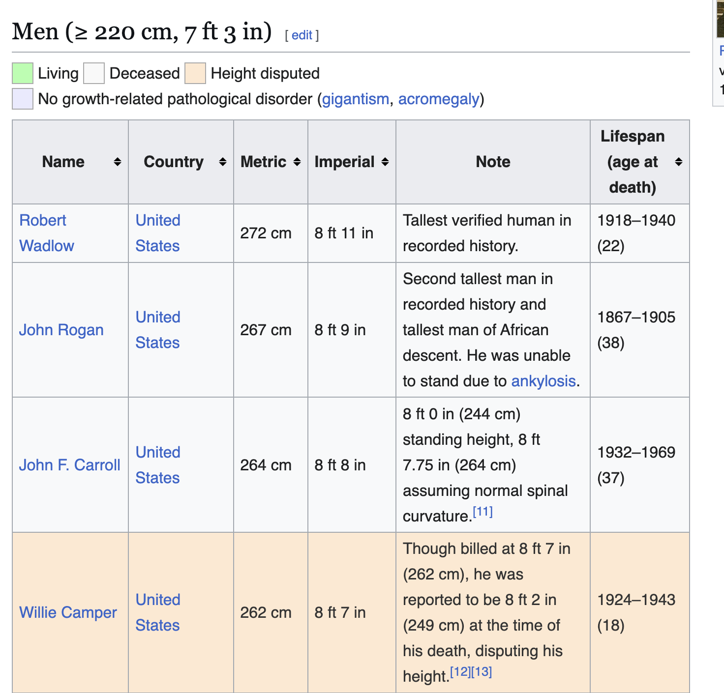
The original table looks like this:
The steps below scrape the data using rvest.
# wikipedia source urlurl <-'https://en.wikipedia.org/wiki/List_of_tallest_people'# grab the first table on the pagetall_table <- url %>%read_html() %>%html_element("table.wikitable") %>%html_table()tall_table <- tall_table %>% janitor::clean_names()tall_table %>%select(c(metric, lifespan_age_at_death, imperial, note))
# A tibble: 219 × 4
   metric lifespan_age_at_death imperial   note
   <chr>  <chr>                 <chr>      <chr>
 1 272 cm 1918–1940 (22)        8 ft 11 in Tallest verified human in recorded h…
 2 267 cm 1867–1905 (38)        8 ft 9 in  Second tallest man in recorded histo…
 3 264 cm 1932–1969 (37)        8 ft 8 in  8 ft 0 in (244 cm) standing height, …
 4 262 cm 1924–1943 (18)        8 ft 7 in  Though billed at 8 ft 7 in (262 cm),…
 5 259 cm 1913–1948 (24–25)     8 ft 6 in  Suffered from Proteus syndrome.
 6 258 cm 1600–1649 (48–49)     8 ft 6 in  Tallest sumo wrestler and first Yoko…
 7 258 cm 1924/25–1944(19–20)   8 ft 6 in  Not officially recognized by Guinnes…
 8 257 cm 1984–2019 (34)        8 ft 5 in  He was reported post mortem to be 9 …
 9 257 cm 1989–2015 (26)        8 ft 5 in  Not recognized by Guinness World Rec…
10 254 cm 1897–1921 (23)        8 ft 4 in  Coyne's World War I draft registrati…
# ℹ 209 more rows
Clearly this requires some data cleaning. Specifically, we need to address the following problems: - The variables metric and imperial mix numbers and text to express height in their respective units - The lifespan_age_at_death variable combines three numeric variables into one column - The note columns often contains reference numbers in brackets
Tidy
1. The metric Variable
First we’ll clean up metric by removing the “cm” on the end of every observation, converting it to a numeric variable, and updating the variable name.
Here we run into our first problem: trailing blanks. When we removed “cm” from the strings, we created phantom blanks, as evidenced by the space between the last digit and the end quote. These will prevent us from cleanly coercing the characters to numbers:
Now we move on to the imperial variable, which takes on the following (un-tidy) values:
tall_table_2$imperial
  [1] "8 ft 11 in" "8 ft 9 in"  "8 ft 8 in"  "8 ft 7 in"  "8 ft 6 in"
  [6] "8 ft 6 in"  "8 ft 6 in"  "8 ft 5 in"  "8 ft 5 in"  "8 ft 4 in"
 [11] "8 ft 3 in"  "8 ft 3 in"  "8 ft 3 in"  "8 ft 3 in"  "8 ft 3 in"
 [16] "8 ft 2 in"  "8 ft 1 in"  "8 ft 1 in"  "8 ft 1 in"  "8 ft 1 in"
 [21] "8 ft 1 in"  "8 ft 0 in"  "8 ft 0 in"  "8 ft 0 in"  "8 ft 0 in"
 [26] "8 ft 0 in"  "8 ft 0 in"  "8 ft 0 in"  "8 ft 0 in"  "8 ft 0 in"
 [31] "7 ft 11 in" "7 ft 11 in" "7 ft 11 in" "7 ft 11 in" "7 ft 11 in"
 [36] "7 ft 11 in" "7 ft 11 in" "7 ft 10 in" "7 ft 10 in" "7 ft 10 in"
 [41] "7 ft 10 in" "7 ft 10 in" "7 ft 10 in" "7 ft 10 in" "7 ft 10 in"
 [46] "7 ft 9 in"  "7 ft 9 in"  "7 ft 9 in"  "7 ft  9 in" "7 ft 9 in"
 [51] "7 ft 9 in"  "7 ft 9 in"  "7 ft 9 in"  "7 ft 9 in"  "7 ft 9 in"
 [56] "7 ft 9 in"  "7 ft 9 in"  "7 ft 9 in"  "7 ft 9 in"  "7 ft 9 in"
 [61] "7 ft 9 in"  "7 ft 9 in"  "7 ft 9 in"  "7 ft 9 in"  "7 ft 9 in"
 [66] "7 ft 9 in"  "7 ft 9 in"  "7 ft 8 in"  "7 ft 8 in"  "7 ft 8 in"
 [71] "7 ft 8 in"  "7 ft 8 in"  "7 ft 8 in"  "7 ft 8 in"  "7 ft 8 in"
 [76] "7 ft 8 in"  "7 ft 8 in"  "7 ft 8 in"  "7 ft 8 in"  "7 ft 8 in"
 [81] "7 ft 8 in"  "7 ft 8 in"  "7 ft 8 in"  "7 ft 7 in"  "7 ft 7 in"
 [86] "7 ft 7 in"  "7 ft 7 in"  "7 ft 7 in"  "7 ft 7 in"  "7 ft 7 in"
 [91] "7 ft 7 in"  "7 ft 7 in"  "7 ft 7 in"  "7 ft 7 in"  "7 ft 7 in"
 [96] "7 ft 7 in"  "7 ft 7 in"  "7 ft 7 in"  "7 ft 7 in"  "7 ft 6 in"
[101] "7 ft 6 in"  "7 ft 6 in"  "7 ft 6 in"  "7 ft 6 in"  "7 ft 6 in"
[106] "7 ft 6 in"  "7 ft 6 in"  "7 ft 6 in"  "7 ft 6 in"  "7 ft 6 in"
[111] "7 ft 6 in"  "7 ft 6 in"  "7 ft 6 in"  "7 ft 6 in"  "7 ft 6 in"
[116] "7 ft 6 in"  "7 ft 6 in"  "7 ft 6 in"  "7 ft 6 in"  "7 ft 6 in"
[121] "7 ft 6 in"  "7 ft 6 in"  "7 ft 6 in"  "7 ft 6 in"  "7 ft 6 in"
[126] "7 ft 6 in"  "7 ft 6 in"  "7 ft 6 in"  "7 ft 6 in"  "7 ft 5 in"
[131] "7 ft 5 in"  "7 ft 5 in"  "7 ft 5 in"  "7 ft 5 in"  "7 ft 5 in"
[136] "7 ft 5 in"  "7 ft 5 in"  "7 ft 5 in"  "7 ft 5 in"  "7 ft 5 in"
[141] "7 ft 5 in"  "7 ft 5 in"  "7 ft 5 in"  "7 ft 5 in"  "7 ft 5 in"
[146] "7 ft 5 in"  "7 ft 5 in"  "7 ft 4 in"  "7 ft 4 in"  "7 ft 4 in"
[151] "7 ft 4 in"  "7 ft 4 in"  "7 ft 4 in"  "7 ft 4 in"  "7 ft 4 in"
[156] "7 ft 4 in"  "7 ft 4 in"  "7 ft 4 in"  "7 ft 4 in"  "7 ft 4 in"
[161] "7 ft 4 in"  "7 ft 4 in"  "7 ft 4 in"  "7 ft 4 in"  "7 ft 4 in"
[166] "7 ft 4 in"  "7 ft 4 in"  "7 ft 3 in"  "7 ft 3 in"  "7 ft 3 in"
[171] "7 ft 3 in"  "7 ft 3 in"  "7 ft 3 in"  "7 ft 3 in"  "7 ft 3 in"
[176] "7 ft 3 in"  "7 ft 3 in"  "7 ft 3 in"  "7 ft 3 in"  "7 ft 3 in"
[181] "7 ft 3 in"  "7 ft 3 in"  "7 ft 3 in"  "7 ft 3 in"  "7 ft 3 in"
[186] "7 ft 3 in"  "7 ft 3 in"  "7 ft 3 in"  "7 ft 3 in"  "7 ft 3 in"
[191] "7 ft 3 in"  "7 ft 3 in"  "7 ft 3 in"  "7 ft 3 in"  "7 ft 3 in"
[196] "7 ft 3 in"  "7 ft 3 in"  "7 ft 3 in"  "7 ft 3 in"  "7 ft 3 in"
[201] "7 ft 3 in"  "7 ft 3 in"  "7 ft 3 in"  "7 ft 3 in"  "7 ft 3 in"
[206] "7 ft 3 in"  "7 ft 3 in"  "7 ft 3 in"  "7 ft 3 in"  "7 ft 3 in"
[211] "7 ft 3 in"  "7 ft 3 in"  "7 ft 3 in"  "7 ft 3 in"  "7 ft 3 in"
[216] "7 ft 3 in"  "7 ft 3 in"  "7 ft 3 in"  "7 ft 3 in"
We’ve got numbers with brackets (links to footnotes in the original Wikipedia page), we’ve got some inches measures that look like “1.5 inches”, some that look like “1+1/2 in”, we have some that drop the plus (“81/2 in”, which should probably read “8 1/2 in”), and then we have one observation that seems to have carried over some style code.
First we’ll fix the style code observation by manually overwriting the value using the original table. We’ll also manually fix the observation that lists a height range (“8 ft 0 in-8 ft 1 in”) since for our purposes, there’s not much difference between an 8-foot person and an 8-foot-one person - they’re both very, very tall.
# manual fixestall_table_3 <- tall_table_2 %>%mutate(imperial =case_when(name =="Rafael França do Nascimento"~"7 ft 8+1⁄3 in", name =="James Toller"~"8 ft 0 in", TRUE~ imperial) , imperial =str_trim(imperial, side ="both") )tall_table_3$imperial
  [1] "8 ft 11 in"    "8 ft 9 in"     "8 ft 8 in"     "8 ft 7 in"
  [5] "8 ft 6 in"     "8 ft 6 in"     "8 ft 6 in"     "8 ft 5 in"
  [9] "8 ft 5 in"     "8 ft 4 in"     "8 ft 3 in"     "8 ft 3 in"
 [13] "8 ft 3 in"     "8 ft 3 in"     "8 ft 3 in"     "8 ft 2 in"
 [17] "8 ft 1 in"     "8 ft 1 in"     "8 ft 1 in"     "8 ft 1 in"
 [21] "8 ft 1 in"     "8 ft 0 in"     "8 ft 0 in"     "8 ft 0 in"
 [25] "8 ft 0 in"     "8 ft 0 in"     "8 ft 0 in"     "8 ft 0 in"
 [29] "8 ft 0 in"     "8 ft 0 in"     "7 ft 11 in"    "7 ft 11 in"
 [33] "7 ft 11 in"    "7 ft 11 in"    "7 ft 11 in"    "7 ft 11 in"
 [37] "7 ft 11 in"    "7 ft 10 in"    "7 ft 10 in"    "7 ft 10 in"
 [41] "7 ft 10 in"    "7 ft 10 in"    "7 ft 10 in"    "7 ft 10 in"
 [45] "7 ft 10 in"    "7 ft 9 in"     "7 ft 9 in"     "7 ft 9 in"
 [49] "7 ft  9 in"    "7 ft 9 in"     "7 ft 9 in"     "7 ft 9 in"
 [53] "7 ft 9 in"     "7 ft 9 in"     "7 ft 9 in"     "7 ft 9 in"
 [57] "7 ft 9 in"     "7 ft 9 in"     "7 ft 9 in"     "7 ft 8+1⁄3 in"
 [61] "7 ft 9 in"     "7 ft 9 in"     "7 ft 9 in"     "7 ft 9 in"
 [65] "7 ft 9 in"     "7 ft 9 in"     "7 ft 9 in"     "7 ft 8 in"
 [69] "7 ft 8 in"     "7 ft 8 in"     "7 ft 8 in"     "7 ft 8 in"
 [73] "7 ft 8 in"     "7 ft 8 in"     "7 ft 8 in"     "7 ft 8 in"
 [77] "7 ft 8 in"     "7 ft 8 in"     "7 ft 8 in"     "7 ft 8 in"
 [81] "7 ft 8 in"     "7 ft 8 in"     "7 ft 8 in"     "7 ft 7 in"
 [85] "7 ft 7 in"     "7 ft 7 in"     "7 ft 7 in"     "7 ft 7 in"
 [89] "7 ft 7 in"     "7 ft 7 in"     "7 ft 7 in"     "7 ft 7 in"
 [93] "7 ft 7 in"     "7 ft 7 in"     "7 ft 7 in"     "7 ft 7 in"
 [97] "7 ft 7 in"     "7 ft 7 in"     "7 ft 7 in"     "7 ft 6 in"
[101] "7 ft 6 in"     "7 ft 6 in"     "7 ft 6 in"     "7 ft 6 in"
[105] "7 ft 6 in"     "7 ft 6 in"     "7 ft 6 in"     "7 ft 6 in"
[109] "7 ft 6 in"     "7 ft 6 in"     "7 ft 6 in"     "7 ft 6 in"
[113] "7 ft 6 in"     "7 ft 6 in"     "7 ft 6 in"     "7 ft 6 in"
[117] "7 ft 6 in"     "7 ft 6 in"     "7 ft 6 in"     "7 ft 6 in"
[121] "7 ft 6 in"     "7 ft 6 in"     "7 ft 6 in"     "7 ft 6 in"
[125] "7 ft 6 in"     "7 ft 6 in"     "7 ft 6 in"     "7 ft 6 in"
[129] "7 ft 6 in"     "7 ft 5 in"     "7 ft 5 in"     "7 ft 5 in"
[133] "7 ft 5 in"     "7 ft 5 in"     "7 ft 5 in"     "7 ft 5 in"
[137] "7 ft 5 in"     "7 ft 5 in"     "7 ft 5 in"     "7 ft 5 in"
[141] "7 ft 5 in"     "7 ft 5 in"     "7 ft 5 in"     "7 ft 5 in"
[145] "7 ft 5 in"     "7 ft 5 in"     "7 ft 5 in"     "7 ft 4 in"
[149] "7 ft 4 in"     "7 ft 4 in"     "7 ft 4 in"     "7 ft 4 in"
[153] "7 ft 4 in"     "7 ft 4 in"     "7 ft 4 in"     "7 ft 4 in"
[157] "7 ft 4 in"     "7 ft 4 in"     "7 ft 4 in"     "7 ft 4 in"
[161] "7 ft 4 in"     "7 ft 4 in"     "7 ft 4 in"     "7 ft 4 in"
[165] "7 ft 4 in"     "7 ft 4 in"     "7 ft 4 in"     "7 ft 3 in"
[169] "7 ft 3 in"     "7 ft 3 in"     "7 ft 3 in"     "7 ft 3 in"
[173] "7 ft 3 in"     "7 ft 3 in"     "7 ft 3 in"     "7 ft 3 in"
[177] "7 ft 3 in"     "7 ft 3 in"     "7 ft 3 in"     "7 ft 3 in"
[181] "7 ft 3 in"     "7 ft 3 in"     "7 ft 3 in"     "7 ft 3 in"
[185] "7 ft 3 in"     "7 ft 3 in"     "7 ft 3 in"     "7 ft 3 in"
[189] "7 ft 3 in"     "7 ft 3 in"     "7 ft 3 in"     "7 ft 3 in"
[193] "7 ft 3 in"     "7 ft 3 in"     "7 ft 3 in"     "7 ft 3 in"
[197] "7 ft 3 in"     "7 ft 3 in"     "7 ft 3 in"     "7 ft 3 in"
[201] "7 ft 3 in"     "7 ft 3 in"     "7 ft 3 in"     "7 ft 3 in"
[205] "7 ft 3 in"     "7 ft 3 in"     "7 ft 3 in"     "7 ft 3 in"
[209] "7 ft 3 in"     "7 ft 3 in"     "7 ft 3 in"     "7 ft 3 in"
[213] "7 ft 3 in"     "7 ft 3 in"     "7 ft 3 in"     "7 ft 3 in"
[217] "7 ft 3 in"     "7 ft 3 in"     "7 ft 3 in"
Next, we’ll remove the un-needed reference numbers in brackets. We can do that manually, too, but it’s not exactly a big-data approach, so let’s use regular expressions (regexps) instead.
The challenge here is that brackets are a special character in regex, so we’ll need to “escape” them (meaning, get R to understand that we mean a literal bracket). The stringrcheat sheet serves as a great summary. You’ll notice that to escape a bracket, you need a double backslash in front of it.
Next, we need to separate the feet and inches values so we can convert to a value like XX.XX inches, allowing us to do numerical manipulation on the value. The pattern in imperial is now “X ft XX in”, where the inches are expressed in different ways (1/2, 0.5). Let’s do inches first. We want to extract out the number that lies between “ft” and “in”. For this, we can use “look around” regexps, that find a pattern preceding or following another pattern. Roughly speaking: - “a(?=c)” means “a” followed by “c” - “(?<=b)a” means “a” preceded by “b” - Note that “[:graph:]” means any letter, number, or punctuation, and the asterisk after it means repeated zero ore more times.
# A tibble: 219 × 2
   imperial   inches
   <chr>      <chr>
 1 8 ft 11 in " 11 "
 2 8 ft 9 in  " 9 "
 3 8 ft 8 in  " 8 "
 4 8 ft 7 in  " 7 "
 5 8 ft 6 in  " 6 "
 6 8 ft 6 in  " 6 "
 7 8 ft 6 in  " 6 "
 8 8 ft 5 in  " 5 "
 9 8 ft 5 in  " 5 "
10 8 ft 4 in  " 4 "
# ℹ 209 more rows
# extract inches value and remove everything from "ft" onward tall_table_5 <- tall_table_4 %>%mutate(inches =str_extract(imperial, "(?<=ft)\\s[:graph:]*\\s(?=in)"),imperial =str_remove(imperial, "\\s(ft)\\s[:graph:]*\\s[:graph:]*")) %>%rename(ht_ft = imperial)# trim white-spacetall_table_6 <- tall_table_5 %>%mutate(inches =str_trim(inches, side =c("both")), ht_ft =str_trim(ht_ft, side =c("both")))
Now, we get to the most challenging part: transforming inches into a numerical variable. This means converting numbers written as fractions into decimals, while not transforming the already-clean decimal values. The simplest way to do this is probably to find a forward-slash (/), and find the numbers immediately before and after it. After that, we’ll separate out the numbers and divide them to arrive at a final, numerical inches_decimal.
Finally, we will add inches to inches_decimal to arrive at the final portion of height in inches. We’ll also address the outlier “7¼” inches. Then, we’ll convert the now-clean inches to feet, and add it to ht_ft.
Now we can do a fun exercise - we can check our work by directly converting ht_cm to height in feet (one foot is 30.48 cm), and seeing if all the wrangling we underwent with inches and feet gave us correct numbers.
# test whether calculated value matches string extracttest <- tall_table_8 %>%select(ht_ft, ht_cm) %>%mutate(check_ht =round(ht_ft*30.48, digits =2))test
We’re not dead on, but we got pretty close. The reason for the error has a lot more to do with rounding in the original table than our text-parsing. And after all that work, our data-frame is tidy-ish.
2. The lifespan_age_at_death Variable
This is what the lifespan_age_at_death column looks like now:
We want the year of birth, year of death, and age at death to be their own variables. Scanning the values, there are several different scenarios: 1. Birth year - death year (YYYY-YYYY) followed by (age or age range) 2. Range for birth year and death year (YYYY/YY - YYYY/YY) 3. “born” followed by a year of birth (YYYY) and no death year 4. Some text followed by “?” followed by a year 5. Year of birth 6. “born” followed by a range and some text 7. Some entries contain a reference number in brackets
First we’ll remove brackets and anything between them, addressing scenario 7. Then we’ll populate an age_at_death variable by extracting anything in parentheses.
# define regular expression for any string between parentheses, not including a parenthesisregex_bet_paren <-"\\([^)]+\\)"tall_table_9 <- tall_table_8 %>%mutate(lifespan_age_at_death =str_remove_all(lifespan_age_at_death, "\\[\\d*\\]"), age_at_death =str_extract(lifespan_age_at_death, regex_bet_paren), lifespan_age_at_death =str_remove_all(lifespan_age_at_death, regex_bet_paren),age_at_death =str_remove_all(age_at_death, "\\(|\\)"), lifespan_age_at_death =str_trim(lifespan_age_at_death, side ="both"),age_at_death =str_trim(age_at_death, side ="both"), age_at_death =if_else(age_at_death =="aged 24 as of March 2022", "", age_at_death) )
Next we separate birth year and death year by the hyphen delimiter. Note the regexp meanings: - \\d* means any quantity of consecutive digits - (?=–) means something followed by a hyphen - (?<=–) means something following a hyphen
Next we’ll address scenario 3: “born” followed by a year of birth (YYYY) and no death year. We’ll also make some manual fixes for a few observtions that don’t translate using our rules.
# populate birth year using a number preceded by "born"tall_table_11 <- tall_table_10 %>%mutate(birth_year =if_else(is.na(birth_year), str_extract(lifespan_age_at_death, "(?<=born )\\d*"), birth_year))
# A tibble: 125 × 3
   lifespan_age_at_death birth_year death_year
   <chr>                      <dbl>      <dbl>
 1 born 1982                   1982         NA
 2 born 1982                   1982         NA
 3 born 1987                   1987         NA
 4 born 1983                   1983         NA
 5 1835–?                      1835         NA
 6 born 1999                   1999         NA
 7 born 1966                   1966         NA
 8 born 1999                   1999         NA
 9 born 1988                   1988         NA
10 born 1986                   1986         NA
# ℹ 115 more rows
3. The note Variable
Finally, we’ll clean up note by removing anything between brackets.
That’s more or less all there is to it. If you’re working with big data, it’ll be a lot more challenging to account for all the patterns. But this example gives us an entry point to regular expressions and using them within the context of stringr.